1.4. Corner Detection#
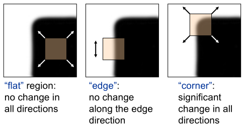
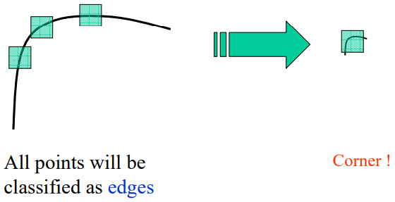
Motivation: shifting a window W in any direction should give a large change in intensity.
Math background#
Correlation#
Given \(\textbf{f - image, h - kernel}\)
cross correlation
auto correlation
Normalized cross correlation
Summed square difference (SSD)#
This is used in template matching. See Correspondence Matching
Relation between SSD and cross correlation#
Harris Corner Detection#
Error function#
Change in appearance of window \(w\) for the shift \((u, v)\):
First-order Taylor approximation for small shifts \((u, v)\) :
Let’s plug this into \(E(u, v)\):
Second moment matrix#
This matrix is weighted sum of nearby gradient information (could use Gaussian weighting).
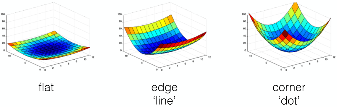
Visualization of a quadratic#
From previous section, \(E(u, v)\) is locally approximated by a quadratic form.
Since \(M\) is symmetric, \(M\) could be diagonalized as
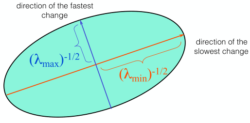
Ellipse equation
Visualize \(M\) as an ellipse with axis lengths determined by the eigenvalues and orientation determined by \(R\)
Eigenvalues interpretation#
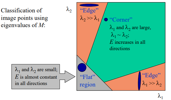
Take-away
\(\lambda_{1}\) and \(\lambda_{2}\) both small: no gradient
\(\lambda_{1} \gg \lambda_{2}\) : gradient in one direction
\(\lambda_{1}\) and \(\lambda_{2}\) similarly large: multiple gradient directions, corner
Threshold on a function of eigenvalues#
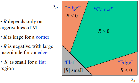
Corner response \(R\)
If these estimates are large, \(\lambda_{1}\) and \(\lambda_{2}\) are similarly large.
Summary#
Source code: C++ and Python implementation.
Intensity change in direction [u,v] can be expressed as a bilinear form:
Compute corner response for each point in terms of eigenvalues of \(M\)
A good corner should have a large intensity change in all directions, i.e. R should be large positive.
Pipeline
Compute partial derivatives \(I_{x}\) and \(I_{y}\) at each pixel
Compute products of derivatives at every pixel
Compute the sums of the products of derivatives at each pixel
Compute second moment matrix \(M\) in a Gaussian window around each pixel
Compute corner response function \(R=\operatorname{det}(M)-\alpha \operatorname{trace}(M)^{2}\)
Threshold \(R\)
Find local maxima of response function (NMS)
Implementaion in Jupyter#
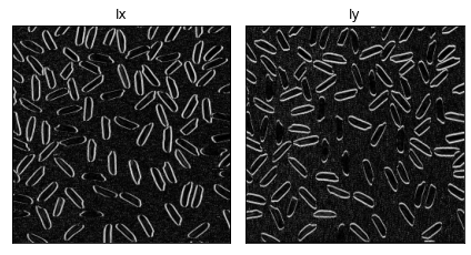
Step1: Image gradients#
image = io.imread(fname="../../data/ass3/rice.png")
h,w = image.shape
# keep the output datatype to some higher forms
Ix = cv.Sobel(image,cv.CV_64F,1,0,ksize=1)
abs_Ix = np.absolute(Ix)
Ix_8u = np.uint8(abs_Ix)
Iy = cv.Sobel(image,cv.CV_64F,0,1,ksize=1)
abs_Iy = np.absolute(Iy)
Iy_8u = np.uint8(abs_Iy)

subplots([Ix_8u, Iy_8u], ['Ix', 'Iy'], 1,2)
Step2: Second movement matrix M#
# Gaussian truncate window
kernel_size = 3
sigma = 0.5
Ixx = cv.GaussianBlur(Ix**2,(kernel_size,kernel_size), sigma)
Ixy = cv.GaussianBlur(Ix*Iy,(kernel_size,kernel_size), sigma)
Iyy = cv.GaussianBlur(Iy**2,(kernel_size,kernel_size), sigma)
Step3: Compute corner response function R#
offset = np.int8(kernel_size/2)
height, width = image.shape
corner_response = np.zeros((height, width))

# construct matrix elements
k = 0.02
for y in range(offset, height-offset):
    for x in range(offset, width-offset):
        A = np.sum(Ixx[y-offset:y+1+offset, x-offset:x+1+offset])
        C = np.sum(Iyy[y-offset:y+1+offset, x-offset:x+1+offset])
        B = np.sum(Ixy[y-offset:y+1+offset, x-offset:x+1+offset])
        det = (A * C) - (B**2)
        trace = A + C
        R = det - k*(trace**2)
        corner_response[y][x] = R
Step4: Corner response calculation and Non-maximum suppression#
# Response threshold 0.2*r_max
R_max = np.max(corner_response)
Threshold_mask = corner_response > 0.2*R_max
# Non max suppression mask
NMS_mask = (corner_response == maximum_filter(corner_response, 5))
mask = Threshold_mask & NMS_mask
keypoints = np.argwhere(mask==True)

# compare with open source library
# keypoints = corner_peaks(corner_harris(image), min_distance=5, threshold_rel=0.02)
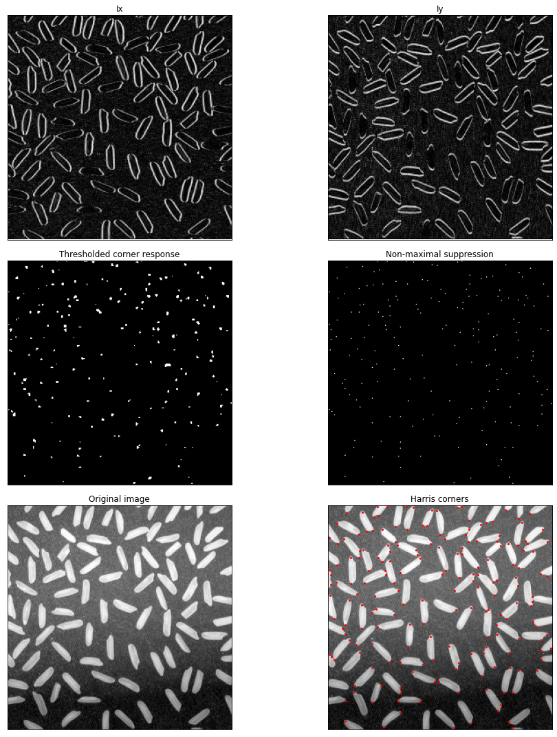
Intermediate results visualization#
Show code cell source
plt.figure(figsize=(15, 15))
imgs =  [Ix_8u, Iy_8u, Threshold_mask, mask, image]
titles = ['Ix', 'Iy', 'Thresholded corner response', 'Non-maximal suppression', 'Original image']

for i in range(5):
  plt.subplot(3,2,i+1),plt.imshow(imgs[i],'gray')
  plt.title(titles[i])
  plt.xticks([]),plt.yticks([])

plt.subplot(3,2,6)
plt.imshow(imgs[-1], cmap=plt.cm.gray)
plt.plot(keypoints[:, 1], keypoints[:, 0], color='red', marker='o',
        linestyle='None', markersize=2)
plt.title('Harris corners')
plt.xticks([]),plt.yticks([])
plt.tight_layout()
plt.show()
Invariance discussion#
Rotation invariance#
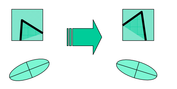
Corner response R is invariant to image rotation
Since Ellipse rotates but its shape (i.e. eigenvalues) remains the same.
Photometric transformations#
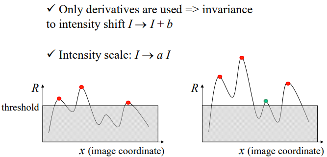
Partial invariance to additive and multiplicative intensity changes
Not invariant to changes in contrast.
Scale invariance#
Not invariant to scaling
Blob detection with Laplacian kernel could solve this.