1.6. 2D transformations

After the feature detection and description, we need to figure out transform between images

• how can we transform images?

• how do we solve for this transformation in given matches?

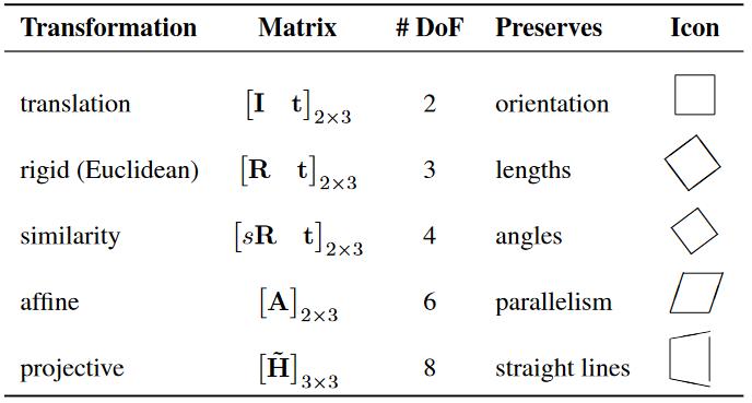
2D planar transformations

Details from NUS CS4243 Computer Vision and Pattern Recognition

Table 1.1 Basic matrix transform

Scaling	Rotation	Translation \(\overline{\mathbf{x}}\)
\[\begin{split} \left[\begin{array}{ll} s_{x} & 0 \\ 0 & s_{y} \end{array}\right] \end{split}\]	\[\begin{split} \left[\begin{array}{cc} \cos \theta & -\sin \theta \\ \sin \theta & \cos \theta \end{array}\right] \end{split}\]	\[\begin{split} \left[\begin{array}{ccc} 1 & 0 & t_ \mathbf{x} \\ 0 & 1 & t_ \mathbf{y} \end{array}\right] \end{split}\]

Table 1.2 Combinations of basic transformations

Euclidean	Similarity	Affine
\[\begin{split} \left[\begin{array}{cc} \mathbf{R} & \mathbf{t} \\ \mathbf{0} & 1\end{array}\right] \end{split}\]	\[\begin{split} \left[\begin{array}{cc}s \mathbf{R} & \mathbf{t} \\ \mathbf{0} & 1\end{array}\right] \end{split}\]	shear + similarity
\[\begin{split} \left[\begin{array}{ccc}\cos \theta & -\sin \theta & t_{x}\\ \sin \theta & \cos \theta & t_{y}\\ 0 & 0 & 1 \end{array}\right] \end{split}\]	\[\begin{split} \left[\begin{array}{ccc}a & -b & t_{x} \\ b & a & t_{y} \\ 0 & 0 & 1 \end{array}\right] \end{split}\]	\[\begin{split} \left[\begin{array}{ccc} a_{11} & a_{12} & a_{13} \\ a_{21} & a_{22} & a_{23} \\ 0 & 0 & 1 \end{array}\right] \end{split}\]

Intro of Homogeneous Coordinates

Introduction of \(\overline{\mathbf{p}} = (x, y, 1)\) in translation

Excellent videos: Projective geometry from UNSW Prof NJ Wildberger

Interesting phenomenons originated from this

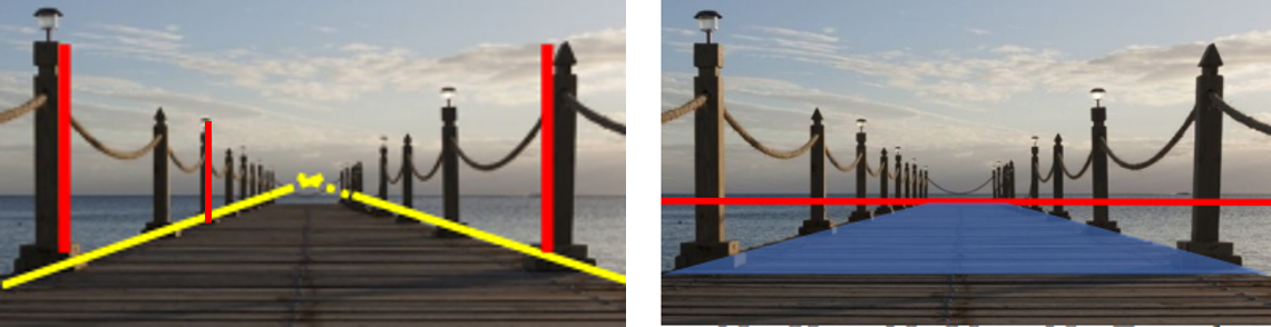
1. Farther away objects are smaller

\[\frac{Y}{Z^{\prime}} < \frac{Y}{Z}, \text{where } Z^{\prime} > Z\]

2. Parallel lines converge at a point.

3. Parallel planes converge! 消失的地平线

Cartesian -> Homogeneous

Understand the 2D projection in the 3D homogeneous coordinate.

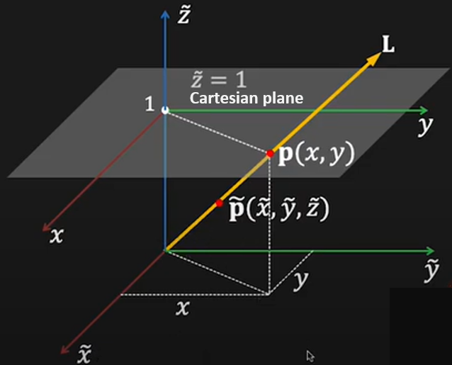Cartesian plane overlaid in the homogeneous coordinate

The \(\color{orange}{homogenous}\) (scale invariant) coordinates of a 2D point

\[\begin{split} \mathbf{p} = \left[\begin{array}{c} x \\ y \end{array}\right]\end{split}\]

are

\[\begin{split}\widetilde{\mathbf{p}} = \left[\begin{array}{c} \widetilde{x} \\ \widetilde{y} \\ \widetilde{z} \end{array}\right] \end{split}\]

Image a line from the origin through \(\widetilde{\mathbf{p}}\)

The third coordinate \(\widetilde{z}\) is fictitious(虚构) such that:

\[\begin{split}\mathbf{\widetilde{x}} \equiv\left[\begin{array}{c} \widetilde{x} \\ \widetilde{y} \\ \widetilde{z} \end{array}\right] \equiv \left [\begin{array}{c} \frac{\tilde{x}}{\tilde{z}} \\ \frac{\tilde{y}}{\tilde{z}} \\ 1 \end{array}\right] \Rightarrow {\mathbf{x}} = \left[\begin{array}{l} \frac{\tilde{x}}{\tilde{z}} \\ \frac{\tilde{y}}{\tilde{z}} \end{array}\right] = \left[\begin{array}{l} x\\ y \end{array}\right] \end{split}\]

In case \(\tilde{z}=0\) -> “point at infinity”

The homogenous representation of a 2D line: $\( \mathbf{\widetilde{x} \cdot \mathbf{\widetilde{l}} = ax+by+c=0} \)$

Where \(\mathbf{\widetilde{l}=(a,b,c)}\) could be normalized as \(\mathbf{\widetilde{l}=(\mathbf{n}, d)}\)

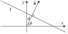2D line equation

Computing homographys

Task: given a set of matching features/points between source and destination images, find the \(\color{orange}{\text{homography H}}\) that best fits.

\[\begin{split}\left[\begin{array}{c}x_{d} \\ y_{d} \\ 1\end{array}\right] \equiv\left[\begin{array}{c}\tilde{x}_{d} \\ \tilde{y}_{d} \\ \tilde{z}_{d}\end{array}\right]=\left[\begin{array}{lll}h_{11} & h_{12} & h_{13} \\ h_{21} & h_{22} & h_{23} \\ h_{31} & h_{32} & h_{33}\end{array}\right]\left[\begin{array}{c}x_{s} \\ y_{s} \\ 1\end{array}\right]\end{split}\]

8 degrees of freedom requires 4 matches. For a given pair i of corresponding points:

\[\begin{split}x_{d}^{(i)}=\frac{\tilde{x}_{d}^{(i)}}{\tilde{z}_{d}^{(i)}}=\frac{h_{11} x_{s}^{(i)}+h_{12} y_{s}^{(i)}+h_{13}}{h_{31} x_{s}^{(i)}+h_{32} y_{s}^{(i)}+h_{33}} \\ y_{d}^{(i)}=\frac{\tilde{y}_{d}^{(i)}}{\tilde{z}_{d}^{(i)}}=\frac{h_{21} x_{s}^{(i)}+h_{22} y_{s}^{(i)}+h_{23}}{h_{31} x_{s}^{(i)}+h_{32} y_{s}^{(i)}+h_{33}} \end{split}\]

Rearrange the terms：

\[\begin{split}x_{d}^{(i)}\left(h_{31} x_{s}^{(i)}+h_{32} y_{s}^{(i)}+h_{33}\right)=h_{11} x_{s}^{(i)}+h_{12} y_{s}^{(i)}+h_{13} \\ y_{d}^{(i)}\left(h_{31} x_{s}^{(i)}+h_{32} y_{s}^{(i)}+h_{33}\right)=h_{21} x_{s}^{(i)}+h_{22} y_{s}^{(i)}+h_{23} \end{split}\]

Linear equation, fixing \(h_{33} = 1\):

\[\begin{split}\left[\begin{array}{cccccccc}x_{s}^{(i)} & y_{s}^{(i)} & 1 & 0 & 0 & 0 & -x_{d}^{(i)} x_{s}^{(i)} & -x_{d}^{(i)} y_{s}^{(i)} \\ 0 & 0 & 0 & x_{s}^{(i)} & y_{s}^{(i)} & 1 & -y_{d}^{(i)} x_{s}^{(i)} & -y_{d}^{(i)} y_{s}^{(i)} \end{array}\right]\left[\begin{array}{l}h_{11} \\ h_{12} \\ h_{13} \\ h_{21} \\ h_{22} \\ h_{23} \\ h_{31} \\ h_{32} \end{array}\right]=\left[\begin{array}{l} x_{d}^{(i)} \\ y_{d}^{(i)}\end{array}\right]\end{split}\]

Normal equation

Solution to \(\mathbf{A x}=\mathbf{b}\):

\[\mathbf{x}=\left[\mathbf{A}^{\mathbf{T}} \mathbf{A}\right]^{-\mathbf{1}} \mathbf{A}^{\mathbf{T}} \mathbf{b}\]

• \(\mathbf{A}\) is not square and so has no inverse.

• \(\left[\mathbf{A}^{\mathbf{T}} \mathbf{A}\right]^{-\mathbf{1}} \mathbf{A}^{\mathbf{T}}\) is the pseudo-inverse of M

• Pseudo-inverse gives the least squared error solution

SVD explanation

\[ \left\|\mathbf{U S V}^{T} \mathbf{h}\right\|^{2}=\mathbf{h}^{T} \mathbf{V S} \mathbf{S}^{T} \mathbf{U}^{T} \mathbf{U S V}^{T} \mathbf{h}=\mathbf{h}^{T} \mathbf{V} \mathbf{S}^{T} \mathbf{S V}^{T} \mathbf{h}=\left\|\mathbf{S} \mathbf{V}^{T} \mathbf{h}\right\|^{2} \]

Where \(\mathbf{A}=\mathbf{U S V}^{T}\), \(\mathbf{U}\) and \(\mathbf{V}\) are orthonormal and \(\mathbf{S}\) is diagonal. And the equation could be furthered developed as:

\[\|\mathbf{S} \mathbf{y}\| \text{ subject to } \|\mathbf{y}\|=1 \text{ where } \mathbf{y} = \mathbf{V}^{T} \mathbf{h}\]

Conclusion: Eigenvector \(\mathbf{h}\) with smallest eigenvalue \(\lambda\) of matrix \(A^{T} A\) minimizes the loss function \(L(\mathbf{h})\).
OR since \(\mathbf{S}\) is diagonal and the eigenvalues are sorted in descending order, let \(\mathbf{y}=[0,0, \ldots, 1]^{T}\) would minimize \(\|\mathbf{S y}\|\). So the solution \(\mathbf{h}=\mathbf{V} \mathbf{y}\) would be the last column vector of \(\mathbf{V}\).